Change of Probability Measure

Change of probability measure is a powerful and beautiful technique, though its presentation in textbooks is often initially met with confusion.

In most resources I’ve encountered, the presentation of the topic typically begins with technical results from measure theory, followed by an involved example which is often related to finance.

Whilst this is fine, in my experience I found it difficult to develop a first principles understanding of where the theory comes from. In this post, I aim to go the oposite way; beginning with what is hopefully an accesible example of how one might develop the technique, before diving into a presentation of the actual theory. To close, I present a more complicated and practical applcation in regards to pricing a particular financial derivative.

A Simple Example

Imagine we can readily sample numbers from a $N(0,1)$ distribution, but we require a sample of a $N(\mu, 1)$ . One option is to to take some a sample $z\sim N(0, 1)$ and then set $x = \mu + z$ so that $x\sim N(\mu, 1)$ . In some sense, one can think of this as shifting the outcome of the first distribution to match a sample from our desired distrbution.

Another approach is as follows: Suppose we can sample $z\sim N(0,1)$ but we wish to sample a $N(\mu,1)$ . We know the target distribution has density $f(x|\mu) = \frac{1}{\sqrt{2\pi}} e^{-\frac{(x-\mu)^2}{2}} \tag{1}$ While the distribution we can sanmple from has density

$f_Z(z) = \frac{1}{\sqrt{2\pi}} e^{-\frac{z^2}{2}} \tag{2}$ The densities look quite similiar. In fact,

$\begin{aligned} f(x|\mu) = \frac{1}{\sqrt{2\pi}} e^{-\frac{(x-\mu)^2}{2}} &= \frac{1}{\sqrt{2\pi}} e^{-\frac{1}{2}(x^2-2x\mu+\mu^2)} \\ &= f_Z(x) \cdot e^{x\mu - \frac{\mu^2}{2}} \end{aligned}$

So, if we sample a $z\sim N(0,1)$ then $f_Z(z)\cdot e^{z\mu - \mu^2/2} \stackrel{d}{=} N(\mu, 1)$ as desired.

So what happened here? Instead of shifting the outcome z by some constant, we found we could reweight its density by the amount $\exp(\mu z - \mu^2/2)$ to match the desired probability distribution we were targeting.

The Radon-Nikodym Derivative

If we take a step back and think about probabilities as assinging some volume, representing likelihood of some event $A$ where sits in a space of possible outcomes $A\subseteq \Omega$ ¹, then the probability denoted by $\mathbb{P}(A)$ denotes the volume, or size that $A$ occupies in $\Omega$ .

Here, $\mathbb{P}$ is a measure function, it takes some set $A$ and spits out a corresponding size. In particular $\mathbb{P}$ is a probability measure which means it has the special property that $\mathbb{P}(\cdot)\in[0,1]$ .

In our example we began with a way to sample $N(0,1)$ , which means we have access to a measure $\mathbb{P}$ which assings sizes of sets in accordance to a standard Gaussian distribution. We wanted to swap however, to a different measure $\mathbb{Q}$ , which assinged probability accordining to a $N(\mu, 1)$ random variable.

In our example, we found the precise amount $\Lambda = \exp(\mu z - \mu^2/2)$ to tilt the $\mathbb{P}$ distribution to become $\mathbb{Q}$. This amount, which I denote by $\Lambda$ , has a special name: it’s a Radon-Nikodym derivative, which describe how to move from one measure to another.

The natural questions to ask at this point are; 1. Can we be sure that a Radon-Nikodym derivative exists for any given starting measure $\mathbb{P}$ and target measure $\mathbb{Q}$ ? 2. How can we find the analytical form of Radon-Nikodym derivative $\Lambda$ and 3. How can swap between measures to compute probabilities?

The Radon-Nikodym Theorem from Measure Theory answers the first question precisly for us; so long as for any set $A$ such that $\mathbb{Q}(A)=0$ we have $\mathbb{P}(A)=0$ then there is a unique function $\Lambda$ such that ² $\mathbb{Q}(A) = \int_A \Lambda d\mathbb{P} \tag{*}$ I won’t proceed with a full proof, but I’ll attempt to unpack and intuit why these conditions are necessary, and how one can see that the theorem should hold.

First the condition of the theorem: for any set $A$ such that $\mathbb{Q}(A)=0$ we have $\mathbb{P}(A)=0$ . This type of relationship is special in Measure Theory and even has it’s own name and notation. We say that $\mathbb{Q}$ is absolutely continuous with respect to $\mathbb{P}$ which we denote by $\mathbb{Q}\ll\mathbb{P}$ .

In the context of probability, the absolute continuity requirement states that the target distribution $\mathbb{Q}$ needs to agree with $\mathbb{P}$ on what outcomes are impossible. If we didn’t have this condition, inconsistent outcomes would arise where once impossible events would become possible when switching to a new measure.

Proving that we can always to find a $\Lambda$ in (*) is less straightforward, but the proof follows a constructive argument by taking a sequence of simpler functions $\{\Lambda_n\}$ whose integrals with respect to $\mathbb{P}$ match the desired behaviour. The sequence is constructed such that each successive element gives a more refined measured that captures the distribuition of $\mathbb{Q}$ more closely. In the limit, we can show that equation in * holds. Moreover, since the limit of a sequence is unique, we can immiediately deduce that $\Lambda$ is unique as well.

Finding Radon-Nikodym Derivatives Analytically

Once we have shown that $\mathbb{Q} \ll \mathbb{P}$ finding Radon-Nikodym derivatives aren’t that difficult. Recall that $\mathbb{P}$ is a measure, so we can write the measure of any set $\mathbb{P}(A)$ as the integtal $\mathbb{P}(A) = \int_A d\mathbb{P} \tag{4}$ If you’re not used to seeing an expression like (4), just think that the $d\mathbb{P}$ term means the change in measure $\mathbb{P}$ . For a probability measure, what would this change in measure be? Hopefully after pondering for a few minutes, you would agree that it’s the change in the corresponding distribution function of the measure, $F(A):=\mathbb{P}(A\in dx)$ . So, the change in the distribution function by a small amount is a change in it’s derivative according to change in it’s argument by a small amount. Said more mathematically, $d\mathbb{P} = dF(x) = f(x)dx$ so we can also write (4) as $\mathbb{P}(A) = \int_A d\mathbb{P} = \int_A d F(x) = \int_A f(x)dx$ Going back to Radon-Nikodym derivatives, we know that $\mathbb{Q}(A) = \int_A \Lambda d\mathbb{P}$ and from above, we also have $\mathbb{Q}(A) = \int_A d\mathbb{Q}$ Now it should be obvious that the correct form we need is $\Lambda = \frac{d\mathbb{Q}}{d\mathbb{P}} = \frac{g(x)}{f(x)}$ where $g,f$ are the $\mathbb{Q}, \mathbb{P}$ densitities respectively.

In short, finding Radon-Nikdoym derivatives analytically is quite simple: take your target density $g$ and your starting density $f$ then look at their ratio $g/f$ . We can confirm this by looking at our simple example from before.

Suppose we want to find the Radon-Nikodym derivative to move from $N(0,1)$ to $N(\mu,1)$ , then

$\begin{aligned} \Lambda &= \frac{\frac{1}{\sqrt{2\pi}}\exp(-(x-\mu)^2/2)}{\frac{1}{\sqrt{2\pi}}\exp(-x^2/2)} \\ &= \exp(x\mu - \mu^2/2) \end{aligned}$

Swapping Between Measures

There’s a few reasons in for why you might want to swap between measures. The first scnenario we explored is related to sampling from a target distribution. The other two common reasons are; Firstly, some random process you are interested in studying is more nicely behaved under a different measure, most commonly through becoming a martingale. The other situation is analysis or estimation becomes more tractable when working with a nice distribution.

It’s important to conceptualise that we start with our real-world / actual probability measure $\mathbb{P}$ , then swap to a nicer $\mathbb{Q}$ to perform some calculations. Sometimes, we can’t interpret this $\mathbb{Q}$ measure directly though, so we need to then swap back to $\mathbb{P}$ .

Before closing out with an example, let’s put this all together on how we can seemlessly swap between two measures $\mathbb{Q}, \mathbb{P}$ once we have their Radon-Nikodym Derivative $\Lambda = d\mathbb{Q} / d\mathbb{P}$ .

By Random-Nikodymn theorem, we then know that any $\mathbb{Q}(A)$ can be written as

$\mathbb{Q}(A) = \int_A \Lambda d\mathbb{P} = \mathbb{E_P}[\Lambda \cdot 1_{A}]$

Before closing out with an example, let’s put this all together on how we can seemlessly swap between two measures $\mathbb{Q}, \mathbb{P}$ once we have their Radon-Nikodym Derivative $\Lambda = d\mathbb{Q} / d\mathbb{P}$ .

By Random-Nikodymn theorem, we then know that any $\mathbb{Q}(A)$ can be written as

$\mathbb{Q}(A) = \int_A \Lambda d\mathbb{P} = \mathbb{E_P}[\Lambda \cdot 1_{A}]$

where $1_A$ is the indicator function. Once we’ve calculated the desired probability, we can swap back with an inverted procedure

$\mathbb{P}(A) = \int_A \Lambda^{-1} d\mathbb{Q} = \mathbb{E_Q}[\Lambda^{-1} \cdot 1_{A}]$

An Application to Digital Option Pricing

Let’s depart from mathematics from a second, and turn our attention to finance. We consider a particular type of contract which is traded in the markets called a Digital Call Option.

A Digital Call Option (or henceforth, a Digital Call) struck at price $K>0$ , expiring at future time $T$ gives the holder of the contract a payoff of $1 in the event that some underlying security (eg a stock, bond, currency) closes above the price K at time $T$ .

It’s clear a Digital Call is a bet on the bimodal outcome for some underlying asset price ends up above or below $K$ . The question is, how much would one be willing to pay to make this bet?

Without any formal mathematical finance theory, one approach we could take is to simply estimate the probability $p := \mathbb{P}(S_T > K)$ . We then know by the binary outcome of the contract that the expected payoff is $$1\cdot p$ .

Unfortunately, the probabilites of stock price movements aren’t easily observable, but suppose we know that the terminal value of the asset price follows $S_T\sim U(0,1)$ . From above, we know that the price of the digital call is therefore

$C = \mathbb{E_P}(1_{S_T > K}) = \int_0^{100} 1_{z > K}dz$

Finding the value of this definite integral is cumbersome, so let’s attack the problem with Monte-Carlo. The strategy is to simulate $n$ random variables $U_i\sim U(0,1)$ and then form the estimate

$\hat{C}_n := \frac{1}{n}\sum_{k=1}^{n}1_{U_k > K} \tag{6}$

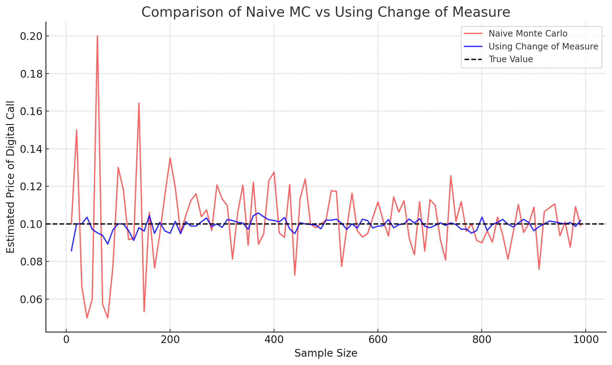
By the law of large numbers, we know that that the right hand side approachs the true price given by the integral as we take $n\to\infty$ . Suppose we’re considering an option that’s struck at $K=0.9$ . Looking at (6), we see that one in every ten samples $U_k$ will have non-zero value; meaning that many of the simulations we conduct will be “wasted”. Moreover, for high value of $K$ the estimator has high variance.

Instead, we can change the measure to place more emphasis on the part of the distribution where the distribution does have value. Let’s define the target measure through the density

$f(x) = \begin{cases} \frac{\alpha}{K} & 0\leq x\leq K \\ \frac{1-\alpha}{1-K} & K\leq x\leq 1 \end{cases} \tag{7}$

for some $\alpha\in(0,1)$ . This density places greater emphasis on the area of where the option has value. Since the $\mathbb{P}$ -density is simple $f(x)=1$ we can obtain the value of the Digital Call option as

$\begin{aligned} C = \mathbb{E_P}(1_{S_T > K}) &= \mathbb{E_Q}\left(1_{S_T>K}\frac{d\mathbb{P}}{d\mathbb{Q}}\right) \\ &= \frac{1-K}{1-\alpha}\mathbb{E_Q}(1_{S_T > K}) \end{aligned}$

which can be estimated via Monte-Carlo through

$\hat{C} = \frac{1-K}{1-\alpha}\frac{1}{n}\sum_{i=0}^{n}1_{U_i^* > K}$

where $U_i^*$ follows the density given by (7). In the plot below, we see the change of measure scheme we proposed above leads to a far more stable, and quicker estimate of the true digital option price.

Footnotes